1. Introduction

Weaving Theory [1] holds that the spacetime geometry of our universe can be described by a three-dimensional four-valent tensor network, i.e. the cubic diamond (3C) net, whose orthogonal projection onto a two-dimensional plane along the stacking axis gives a trivalent (honeycomb) network. The elementary unit of the network, a_P = 2√(ln8)·l_P ([1], Corollary 3), is a binary 3-bit (8-state) quantum entanglement relation. Throughout spacetime such entanglement relations are created and annihilated; because of the constraint of charge conservation, a change in the state of one elementary entanglement relation instantaneously disturbs the whole network, so that the states of other units change in synchrony—this is the phenomenon of quantum entanglement. In a local region of spacetime, the elementary units, constrained by the gauge forces, can form structure-specific entanglement relations in the locked or bound states; matter is thereby emergent [2,3]. The central thesis of this paper is that gravity is not fundamentally a force but the relative gradient of the a_P field density between spacetime and matter. Starting from the underlying structure of spacetime geometry, this paper derives the gravitational equations of Weaving Theory and the unified metric (the density, shear, and drag slots), gives the point-source solution and the strong-field behavior, and compares the surface gravitational acceleration of solar-system bodies and the surface redshift of neutron stars with the results of the Einstein equation, thereby testing the accuracy of the equations.

---

2. The Nature of Gravity

General relativity holds that gravity is not a force but the curvature of spacetime [4]. Matter and energy distort the surrounding spacetime geometry, and bodies move along geodesics in the curved spacetime, so that they appear to attract one another. Light also propagates along geodesics, so that a light ray passing near a massive body is deflected; and because clocks run at different rates at different places in a curved spacetime, light is slowed along the stretch of its path that lies in the gravitational field, arrives with a delay, and is lowered in frequency. This geometric description agrees closely with observation at solar-system scales [5], and “gravity is the curvature of spacetime” has therefore become the standard picture of gravity today. But general relativity does not answer why spacetime should curve, what the origin of gravity really is, or why gravitational waves travel at the speed of light; and at the Planck scale it comes into conflict with quantum mechanics [6].

We hold that the substance of the universe is a superposition of quantum entanglement relations, not matter. a_P is an elementary quantum entanglement relation unit, expressed by binary 3 bits, a superposition of 8 states; hence spacetime geometry and matter are both expressed through the way a_P units are woven. Spacetime is not the background of matter, nor is matter independent of spacetime: matter is formed where a local a_P network reaches a locked or bound state under the constraints of charge conservation and the gauge forces [2,3], while vacuum is spacetime in a state in which the a_P relations fluctuate freely under the charge-conservation constraint. The emergence of matter locks or binds the quantum states of the a_P units of the surrounding spacetime. To exist in spacetime, matter must establish stable entanglement relations with spacetime rather than stand apart from it. Gravity is an intrinsic property of spacetime and matter together, not a property of matter alone. The reason a celestial body stays in a relatively regular orbit in spacetime is that it is pulled by the gravity of the whole spacetime geometry and reaches an equilibrium of gravitational balance with spacetime and with other bodies.

Gravity comes from the counting of a_P units; but the metric read out is different in different energy–momentum settings, so that the metric has to be constructed for each setting separately. The number of a_P locked or bound by matter is an additive integer N, and the amount of matter is precisely this count: mass m = N/a_P, unit mass m₁ = 1/a_P. The a_P field density at the location of matter is denoted ρ, and gravity is the relative gradient of the a_P field density. In order to establish stable entanglement relations with the surrounding spacetime, the a_P units locked or bound by a body at the same time determine the quantum states of the a_P of the surrounding spacetime, forming an a_P field whose strength is set by its mass. The a_P field of the spacetime between bodies is determined by the superposition of their respective masses. Why an apple falls: once it leaves the branch, it must establish stable entanglement relations with the surrounding spacetime, but the a_P units of its surroundings are mostly bound by the Earth, so at every position along its geodesic in the air it cannot establish stable entanglement relations; only after it lands on the Earth's surface does it establish stable entanglement relations with the surrounding spacetime. In vacuum, by contrast, because gravity is uniform all around the apple, it can establish stable entanglement relations with spacetime at any position, and so appears to float.

Take an egg and a stone of the same volume and the same shape: the two contain exactly the same number of a_P units. Why, then, is the stone heavier than the egg? The difference lies in the number of a_P units in the locked state within the two volumes. Every a_P unit carries one share of ln8 of entropy; to put an a_P into the locked state one must pay an equal share of energy—and the color field is precisely the source of this energy (mass). Inside the nucleus of a hydrogen atom, gluons bind the quarks together into a six-membered ring (closed by 6 a_P edges), and the quantum state of every edge is in the locked, stable state [3]. The quantum states of the a_P inside the nucleus determine the quantum fluctuation states outside it; they correlate the excitation of the electron with the rest of the network, so that the electron is continually extinguished and lit up again elsewhere [3]. Hence the more a_P are in the locked state, the fewer the available a_P states, and the stronger the binding of the electron. What an atomic clock counts is exactly such an excitation mode constrained by charge conservation—the hyperfine transition of caesium-133, 9 192 631 770 periods of which make one second. And the more a_P locked by the nucleus, the fewer the available states, the longer the coordinate time needed to complete one period, and the slower the clock—that is, dτ/dt = 1/ρ.

Through the Weaving Formula ([1], Corollary 4), the gravitational constant and the speed of light are locked by one and the same a_P: G = a_P²/(4c·ln8). G and c are two readings of one and the same fabric. On the geometric model a_P = 2√(ln8) is 2.884 lP; in real physics it is a quantum entanglement relation. c is the speed of light, whose original meaning is a purely geometric quantity—the saturation strength of the entropy–area coupling ([1], Corollary 4). As c approaches the thermodynamic saturation limit (c∞ = 1, [1], Theorem 3), this geometric quantity becomes identical with the speed of light, i.e. information can propagate in any direction of the spacetime geometry with the upper bound of one a_P per unit time. Gravity likewise propagates through a_P, and hence the speed of gravitational waves equals the speed of light. Time runs slower near a massive body because, when light passes by, the a_P field density around the massive body is large owing to the curvature of spacetime, so that relative to vacuum light has to cross more a_P units—this is how space causes time to slow down.

3. The Gravitational Equations

3.1 The Set of Gravitational Equations

Units (all derivations from this section on): natural units—ħ = c = 1, length measured in the Planck length l_P, time in l_P/c, mass in m₁ = ħ/(a_P c); the elementary unit of the net is a_P = 2√(ln8)·l_P (value 2.884, [1], Corollary 3). Every formula from §3 on is written in this system of units, with no conversion constants carried in the expressions; where SI units are needed, see the conversion table in §3.5.

The theory of gravity established in this section is written as the following closed set of equations, in three parts—the field equation (determining the field), the source rule (matter into source), and the reading rules (field into geometry and observables)—together with the constant definition and the tensor sector (gravitational waves). Here u ≡ ln ρ is the field variable; ρ(x) is the a_P field density (= the number of a_P in the locked and bound states per unit volume divided by the vacuum a_P field density; in vacuum ρ = 1, and relative to vacuum locking only adds, so ρ ≥ 1); n_lock(x) is the number of a_P in the locked and bound states per unit volume, i.e. the source count; N_lock is the total number of a_P in the locked and bound states at one place (one source) (N_lock = Σ N_p, see §4.2); ρ_m is the mass density; g_μν is the metric reading at the geometric layer, and δ_ij is the metric of three-dimensional flat space.

(1) Field equation (determining the field)

∇²(ln ρ) = −(4π/a_P)·n_lock                                 (3.1)

(2) Source rule (matter into source)

ρ_m = n_lock/a_P                                            (3.2)

Each relation in the locked or bound state contributes one unit of mass m₁ (m₁ = 1/a_P in natural units), hence ρ_m = n_lock/a_P (for the microscopic basis of the source rule see §4.2). Substituting into Eq. (3.1) gives the Poisson form at the geometric layer

∇²(ln ρ) = −(4πG/c²)·ρ_m                                    (3.3)

(3) Reading rules (field into geometry and observables)

ds² = −(1/ρ²) dt² + (ρ² δ_ij + h_ij^TT)(dx^i + N^i dt)(dx^j + N^j dt)        (3.4)

a = c²∇(ln ρ),      1 + z = ρ,      dτ/dt = 1/ρ           (3.5)

Eq. (3.4) is the unified metric: the density slot gives the lapse 1/ρ and the spatial scale ρ²δ_ij, the shear slot gives h_ij^TT (gravitational waves), and the drag slot gives N^i (rotation/translation); the static case (N^i = 0, h_ij^TT = 0) reduces to g₀₀ = −1/ρ² and g_ij = ρ²δ_ij. Eq. (3.5) gives in turn the acceleration, the redshift, and the clock rate; the derivations of the individual slots are given in §6.

(4) Constant and point source

G = a_P²/(4c·ln8)                                           (3.6)

ρ = e^{μ/r},      μ = N_lock/a_P,      g(r) = GM/r²       (3.7)

G is the gravitational constant, its value fixed by a_P ([1], Corollary 4); in natural units G = 1. Eq. (3.7) is the point-source solution of Eqs. (3.1)–(3.3) (μ is the source amplitude, which in natural units is the mass M of the source; the weak field and the strong field share this one expression; for the SI form see §3.5).

(5) Tensor sector (gravitational waves)

(∂_t² − ∇²)h_ij^TT = 0                                      (3.8)

Source-free propagation in vacuum, two polarizations, wave speed c; the coupling constant of the source is G (derivation in §5.1).

How to use it: first count the source—write down n_lock from the matter distribution, or convert from ρ_m by Eq. (3.2); then solve the field—solve the Poisson equation (3.1) for u = ln ρ; finally read—use Eqs. (3.4) and (3.5) to obtain the metric, the acceleration, and the redshift. This set of equations is strictly linear and mutually decoupled: given a source, one only has to solve a single Poisson equation and then read out the geometry and the observables by the reading rules, with no simultaneous iteration. The following sections derive this set of equations one by one.

3.2 The a_P Field Density ρ

The area law S = (L−1)·ln8 ([1], Theorem 1) connects the “geometric quantity” with the “count” (for the established background of the universal area scaling of entanglement entropy see [7–9]): the area A corresponds not to a continuous length squared but to L units of a_P—each a_P carries one unit of area a_P² ([1], Corollary 3):

A = L·a_P²                                                  (3.9)

Hence the a_P field density is defined as

ρ(x) ≡ (number of a_P in the locked and bound states per unit volume)/(vacuum a_P field density)   (3.10)

Each a_P carries one share of ln8 of entropy and is a superposition of 8 quantum states. An a_P in the locked state has its quantum state completely unfree; the locked state directly determines the bound state, i.e. the quantum state of a bound a_P has only limited freedom. In vacuum there are no locked relations—all relations are free and can be freely rearranged—so that the vacuum field density is taken as 1. Relative to vacuum, locking only adds and never subtracts, hence ρ ≥ 1. The larger the number of a_P in the locked state, the larger the field density and the stronger the gravity.

The substance of gravity (the central proposition of this paper):

Gravity is not a force but the relative gradient of the a_P field density.

The acceleration is taken as the relative gradient of this ratio. The field variable u ≡ ln ρ is dimensionless (Eq. (3.13)), so that ∇u has the dimension of an inverse length and can be made into an acceleration only by multiplying by c²; this is also the reading at the geometric layer—u = −Φ/c², a = −∇Φ (§3.3(4)):

a = c²∇(ln ρ) = c²(∇ρ)/ρ                                    (3.11)

In the weak field it reduces to Newtonian gravity (§3.4).

3.3 The Field Equation

Net shape: the three-dimensional network is taken to be the cubic diamond (3C) net—each node is joined by four bonds to four nearest neighbours, the four bond directions pointing to the four vertices of a regular tetrahedron, with mutual angles arccos(−1/3) = 109.4712°; it is formed by two face-centred cubic (fcc) sublattices interpenetrating with a displacement of one quarter along the body diagonal, the bond length being a_P; its standard crystallographic structure is given in [10]. Projecting it orthogonally along the stacking axis gives the trivalent (honeycomb) net—and this planar trivalent net is the one used for the area law. The reason the three-dimensional net is taken to be the cubic diamond (3C) net is that two conditions fix it together: the elementary unit has 4 relations, and the 4 bonds must be equivalent, with the same bond length a_P; the directions of the 4 bonds must be symmetric, otherwise the net is not isotropic, and the unique symmetric solution for the bond angles is the tetrahedral coordination, arccos(−1/3) = 109.4712°. The net satisfying these two conditions and being macroscopically isotropic as a whole is the cubic diamond (3C) net. Its shortest closed loop is the six-membered ring: 6 nodes, 6 bonds (shortest loop length = 6, and it contains no four-membered ring, checked numerically bond by bond). The 6 nodes of a six-membered ring are not strictly coplanar (viewed along the body diagonal they undulate in a chair form). For the discussion of the net shape of spacetime geometry, see The Weaving Formula: Emergence Mechanism of Spacetime Geometry [1].

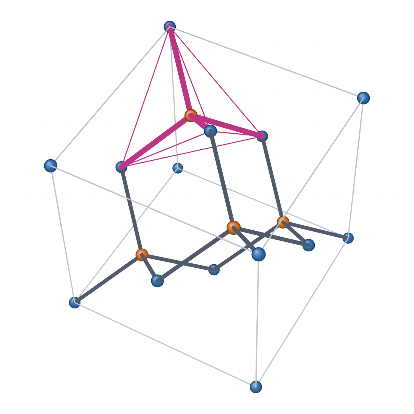
Figure 1. Local detail of the three-dimensional four-valent tensor network, i.e. the cubic diamond (3C) net.

The elementary unit a_P = 2√(ln8)·l_P ([1], Corollary 3), i.e.

a_P² = 4 ln8                                                (3.12)

(1) Field variable. One node is exactly 2³ = 8 states (3 bits), and the contributions of mutually independent bonds multiply ⇒ ln8 is additive over bonds. The source is the number of entanglement relations in the locked and bound states, N—an integer count, additive. The multipole superposition of an additive source requires the field quantity to be additive, and the only additive local scalar is

u ≡ ln ρ                                                    (3.13)

where ρ is the a_P field density (§3.2); each relation that is locked dilutes the available state count by one share, hence ρ ≥ 1.

(2) Four-leg expansion (net → continuum). The unit vectors of the four legs of the tetrahedron satisfy

Σ_a nᵃ = 0,      Σ_a nᵃnᵇ = (4/3)δᵃᵇ                       (3.14)

Writing the four legs as (1,1,1), (1,−1,−1), (−1,1,−1), (−1,−1,1) and normalizing them to unit length: the diagonal element is (1+1+1+1)/3 = 4/3, while the off-diagonal elements vanish by cancellation of signs. Expanding u along each leg to O(a_P²), the linear terms cancel as a whole because Σ_a nᵃ = 0:

u(x + a_P nᵃ) − u(x) ≈ a_P (nᵃ·∇)u + (a_P²/2)(nᵃ·∇)²u
Σ_a (nᵃ·∇)²u = Σ_a nᵃ_α nᵃ_β ∂_α∂_β u = (4/3)∇²u
⇒ Σ_j (u_j − u_i) = (a_P²/2)·(4/3)∇²u = (2/3)a_P²∇²u        (3.15)

(The expansion of Eq. (3.15) is on the three-dimensional four-valent net; the area law is studied on the planar trivalent net; the two layers meet only at the emergent metric (§6).)

(3) Quadratic energy. The elastic strain is taken as a relative change. The density appearing here is counted by volume: ρ_bulk ≡ the ratio of the number of a_P per unit coordinate volume (i.e. the a_P field density, taken as 1 in vacuum; its relation to the line count ρ used elsewhere in this paper is ρ_bulk = ρ³, see §6). Hence the volume allotted to a unit relation ∝ 1/ρ_bulk ⇒ the coordinate lattice-spacing ratio b/b₀ = ρ_bulk^{−1/3}, so that the relative strain is δb/b = −(1/3)ln ρ_bulk. The energy is quadratic in the strain, and written in terms of u = ln ρ it is still a quadratic form, whose stiffness coefficient is the coefficient of Eq. (3.15):

W = (κ_reg/2)∫(∇u)²,      κ_reg = (2/3)a_P²                 (3.16)

(Normalization convention: the gradient operator on a node is given by the four-leg expansion (3.15), i.e. Σ_j(u_j − u_i) = (2/3)a_P²∇²u; taking the coefficient of this operator as the stiffness, κ_reg = (2/3)a_P² (value 5.545177444).) The lattice energy summed over nodes, W = (κ_reg/2)Σ_i(∇u)²·v₁, and its continuum limit (κ_reg/2)∫(∇u)² come from the same relation count (for v₁ see Eq. (3.22)).

(4) Source term and field equation. The source is additive ⇒ the source term can only be linear: W_src = −∫σ·u. The variation δW/δu = 0 gives

∇²u = −σ/κ_reg                                              (3.17)

The source-strength coefficient is fixed by the gravitational constant G. The Poisson reading at the geometric layer is ∇²Φ = 4πGρ_m, and the field variable is related to it by u = −Φ/c² (equivalently a = c²∇u = −∇Φ, Eq. (3.11)); substituting gives

∇²u = −(4πG/c²)·ρ_m                                        (3.18)

Using the source rule ρ_m = n_lock/a_P (§4.2) to write the source as the count at this layer:

∇²u = −(4πG/(c²a_P))·n_lock                                (3.19)

G/c² is a pure number: from G = a_P²/(4c·ln8) of [1], Corollary 4, together with Eq. (3.12),

G/c² = a_P²/(4c³·ln8) = l_P²/c³ = 1      (natural units)     (3.20)

hence 4πG/(c²a_P) = 4π/a_P—the source-strength coefficient is G (written as a mass-density source this is Eq. (3.28)). Also σ = σ₁·n_lock with σ₁ = (4π/a_P)·κ_reg = (8π/3)a_P = 24.161392390530, so that

∇²u = −(4π/a_P)·n_lock                                     (3.21)

(5) Node volume and lattice form. The edge of the diamond unit cell is a = 4a_P/√3 and the cell contains 8 nodes, so that the volume corresponding to each node is

v₁ = a³/8 = 8a_P³/(3√3)                                    (3.22)

The number of relations locked on node i is N_i = n_lock·v₁; substituting ∇²u of Eq. (3.21) into Eq. (3.15):

Σ_j (u_j − u_i) = −q·N_i                                   (3.23)
q = (8π/3)a_P/v₁ = π√3/(4 ln8)      (q = 0.654189836987)

q is the conversion factor that turns the continuum coefficient into a lattice count (per relation, per unit volume). Conversely, substituting N_i = n_lock·v₁ into Eq. (3.23) and using Eqs. (3.12) and (3.22):

∇²u = −(4q/√3)·a_P·n_lock = −(4π/a_P)·n_lock                (3.24)

which returns to the coefficient of Eq. (3.21) (that is, to the field equation (3.1) of §3.1). But this is an algebraic identity, not an independent check: substituting q and a_P² = 4 ln8, (4q/√3)·a_P = (4/√3)·(π√3/(4 ln8))·a_P = π·a_P/ln8 = 2π/√(ln8) = 4π/a_P (value 4.35719012284867); it only shows that the lattice form and the continuum form come from the same relation count. The PPN parameters are given by the same ρ: the clock reading gives g₀₀ = −1/ρ² and the geometry gives g_ij = ρ²δ_ij, and expanding ρ = 1 + U gives γ = β = 1 (§6, §7.1).

3.4 Point-Source Solution

Point source: N_lock relations that are not completely free at a single lattice node, n_lock = N_lock·δ³(x). Integrating ∇²u = −(4π/a_P)·N_lock·δ³(x) directly with ∇²(1/r) = −4πδ³(x):

ln ρ = N_lock/(a_P · r)      ⟹      ρ(r) = e^{μ/r},   μ = N_lock/a_P    (3.25)

In the language of observation: by the source rule (§4.2) the source amplitude is μ = N_lock/a_P, and N_lock/a_P is exactly the mass M of the source; in natural units G = 1 (Eq. (3.20)), so that the acceleration read out from Eq. (3.11) is

g(r) = GM/r²                                                (3.26)

The weak field and the strong field share this one expression; in SI units μ = GM/c² (Eq. (3.29)).

3.5 Conversions to SI Units

The equations before this section (§3.1–§3.4) are written throughout in natural units (ħ = c = 1, length in l_P, time in l_P/c, mass in m₁ = ħ/(a_P c)), with no conversion constants in the expressions. Below, the powers of c and ħ are restored on dimensional grounds and the expressions are written in SI units—length, time, and mass being converted by l_P, l_P/c, and ħ/(a_P c) respectively.

Acceleration         a = c²∇(ln ρ) = c²(∇ρ)/ρ                   (3.27)
Field equation       ∇²(ln ρ) = −(4πG/c²)·ρ_m                   (3.28)
Point source         μ = GM/c²,   ρ = e^{μ/r},   g(r) = GM/r²      (3.29)
Gravitational const. G = a_P²c³/(4ħ·ln8) = l_P²c³/ħ             (3.30)

These are in turn the SI forms of Eqs. (3.11), (3.21), and (3.25)–(3.26); the mass unit is m₁ = ħ/(a_P c). The natural-unit form of [1], Corollary 4, is G = a_P²/(4c·ln8).

Numerical example (SI units): g = GM/R² gives ≈ 274.2 m/s² for the Sun and ≈ 9.82 m/s² for the Earth, in agreement with observation (self-consistency check, §7).

---

4. The Source: the Number of a_P Relations Whose Quantum State Is Not Completely Free

4.1 Matter

The equation ∇²(ln ρ) = −(4π/a_P)·n_lock has only one source: n_lock. What is it?

a_P is the elementary unit of spacetime geometry, and every a_P carries one share of ln8 of entropy. The degree of quantum entanglement of an a_P therefore falls into three cases—completely locked, not completely free, and completely free; and the locked state directly determines the state that is not completely free. In other words, an a_P in the locked state binds the quantum states of the a_P around it, putting them into the state that is not completely free. Hence n_lock is the count, per unit volume, of a_P in the locked state together with those thereby bound. In vacuum the quantum states of a_P are completely free. Inside matter the a_P are in the locked and not-completely-free states, and the mass of matter is contributed mainly by the a_P in the locked state. n_lock is not energy, not momentum, not any external input—it is the only source of the equation.

4.2 The Source Rule

n_lock and the mass differ only by the single scale a_P:

ρ_m = n_lock / a_P                                          (4.1)

N_lock = Σ N_p,   N_p = m/m₁
(m the mass, m₁ the mass unit; from the same relation count as the mass; N_p the mass fraction number of a single particle)

Equivalent reading (from the same relation count as the a_P field density reading, [1], Corollary 3): mass = m₁ × mass fraction number; the ratio of mass fraction numbers is given by the internal-phase-space volume reading of The Weaving Origin of the Proton–Electron Mass Ratio [11] (mass ∝ internal phase-space volume), its absolute value being listed as open; and the particle spectrum itself (who is on the spectrum, carrying which charges and colors) is given in The Weaving Structure of the Matter Spectrum [3].

This yields a verifiable corollary: the mass ratio of two particles = the ratio of their source amplitudes = the ratio of their mass fraction numbers. Taking the proton/electron case:

m_p/m_e = 1836.152673440 (observed)                         (4.2)

That is: the source of the gravitational equations reads out exactly the observed mass spectrum; m_p/m_e does not enter the gravitational field equation itself, it enters only the “source”.

4.3 The Unique Scale

Only one fundamental quantity appears throughout: a_P (equal to 2.884 when l_P is taken as the unit, see §3.2). It is at the same time

• the elementary unit a_P, i.e. one quantum entanglement relation (3 bits, 8 states in all) ([1], Corollary 3);
• the conversion rate between n_lock and mass (§4.2);
• the unique mass unit m₁ = 1/a_P.

---

5. The Tensor Sector and the Scalar Sector

The elastic dynamics of the net gives exactly opposite conclusions in the tensor sector and the scalar sector—the tensor sector governs gravitational waves, the scalar sector governs the “force”.

5.1 The Tensor Sector: (∂_t² − ∇²)h_ij^TT = 0

The net has only one energy rule: energy = −ln(number of states) (the state count is a pure number and transforms as a Jacobian under deformation, §5.2). Expanding it on the diamond net yields two kinds of contribution—the bond-length term (the state count depends only on the bond length) and the volume term (the state count ∝ the deformation Jacobian det F). Acting alone, the bond-length term gives C11 = C12, C44 = 0, and shear develops a zero mode ⇒ the transverse speed vanishes and there are no gravitational waves; the elastic-tensor ratio of the volume term is (C11−C12) : C12 : C44 = 2 : 0 : 1. Weaving Theory has no second counting rule: the bond-length term is not an independent term, it is exactly the deformation component of the volume term ⇒ the elastic tensor takes the pure-volume form:

C12 = 0,      C11 = 2C44       (i.e. the point β/α = 1/2)   (5.1)

Dynamical matrix. The two contributions are written as the standard two terms (the bond-stretch–bond-bend expansion of the valence-force-field model [12])—the bond-length term (deviation of the squared bond length) and the bond-angle term (deviation of the squared bond angle); each node has 4 bonds and 6 bond angles, and b′₁, b′₂ are the two deformed bond vectors at the same node (b′ = b + Δu):

W = (α/2) Σ_{bonds} (b′²/a_P² − 1)² + (β/2) Σ_{angles} (b′₁·b′₂/a_P² + 1/3)²       (5.2)

(α and β are the stiffnesses of the bond-length and bond-angle terms; Weaving Theory has only one counting rule ⇒ one takes the pure-volume point β/α = 1/2.) Expanding Eq. (5.2) to second order in the displacements: the bond-length term gives (2α/a_P²)·Σ_bonds (n·Δu)², and the bond-angle term gives (β/2a_P²)·Σ_angles (n₁·Δu₂ + n₂·Δu₁)² (n is a unit bond direction, Δu the difference of the displacements at the two ends of a bond or an angle; the indices of the bond-angle term are cross-paired). Both are quadratic forms in the displacement differences; writing D(q) = Σ_R Φ(R)e^{iq·R} (Φ the force-constant matrix of the quadratic form, R taken up to second neighbours) as a 6×6 dynamical matrix and diagonalizing, the three acoustic eigenvalues are

v² = (2, 2, 4)      (identical along [100], [110], [111])   (5.3)

The double degeneracy corresponds to the two transverse displacements, and the longitudinal branch corresponds to ∇·u. The dimensionless values of v² depend on the normalization of the bond stiffness and of the length unit ((2,2,4) is one such normalization); the physical content is the ratio: the transverse branch is doubly degenerate and v_L²/v_T² = 2 ⇒ c_L/c_T = √2, independent of direction (isotropic). The absolute scale is fixed by the time-scale convention—taking “one tick covers one a_P” as the unit of time, the wave speed of the transverse (physical) branch is fixed to c ([1], Theorem 3, the thermodynamic saturation limit), and the longitudinal branch is √2 c.

Correspondence between the two contributions and the elastic constants: C11, C12, C44 are the three independent constants of cubic-symmetry elasticity (Voigt notation: C11 = ∂²w/∂ε₁², C12 = ∂²w/∂ε₁∂ε₂, C44 = ∂²w/∂ε₄², with w the strain-energy density and ε₄ = 2ε_yz). Decomposing along [100], the pure longitudinal branch has v_L² = C11/ρ_m and the pure transverse branch v_T² = C44/ρ_m; substituting (v_L², v_T²) = (4, 2) of Eq. (5.3) gives C11 = 2C44, and substituting into the isotropy condition C11 − C12 = 2C44 gives C12 = 0. The anisotropy factor (Zener factor [13]) A = 2C44/(C11−C12) = 1 ⇒ macroscopic isotropy; ν = 0 (no Poisson ratio) and c_L/cT = √2 exactly. The same energy, expanded to second order in a uniform small strain and minimized over the relative displacement of the two sublattices A and B in the cell (w = −H{εw}H_{ww}^{−1}ε), gives the elastic-constant ratio C11 : C12 : C44 = 2 : 0 : 1 (the pure volume term (1/2)tr ε² acting alone gives the same ratio: C11 = 1, C12 = 0, C44 = 1/2), consistent with the values above.

The continuum limit (λ = C12 = 0) gives

∂_t²u_i = c_T²(∇²u_i + ∂_i∇·u)                              (5.4)

At the geometric layer the net displacement field is read as strain, h_ij := ∂_i u_j + ∂_j u_i (twice the strain; the bridge is §6); substituting into Eq. (5.4) gives ∂_t²h_ij = c_T²(∇²h_ij + ∂_i∂_j h), and taking the transverse traceless part (∇·u = 0, i.e. the transverse branch):

(∂_t² − ∇²)h_ij^TT = 0                                      (5.5)

That is: source-free propagation in vacuum, two polarizations, wave speed = c_T = c (one tick covering one a_P is the speed of light, [1], Theorem 3, the thermodynamic saturation limit). The longitudinal branch is exactly pure gauge (h_ij = ∂_i u_j + ∂_j u_i is a coordinate transformation) ⇒ the physical spectrum is 2 transverse polarizations, in agreement with the observed degrees of freedom of gravity.

With a source, the tensor-sector equation is

□ h_ij^TT = −κ·τ_ij^TT,      κ = 4π/a_P                      (5.6)

Here κ is the same as the coefficient of the scalar sector, Eq. (3.1) (that is, the G of the geometric layer, §3.3): the source τ_ij = n_lock·⟨n_i n_j⟩ is the directional tensor of the locked relations (⟨·⟩ denotes the average taken over the directions of the locked bonds at that place, n being a unit bond direction), whose trace tr τ = n_lock is the source of the scalar (Newtonian) sector, while its traceless transverse part gives the source of gravitational waves. The tensor sector and the scalar sector use the same counting and the same coupling at the relation layer, with no extra conversion factor; the longitudinal branch is pure gauge, and the physical spectrum has only 2 transverse polarizations.

Why the volume term is necessary: if the elasticity depended only on bond lengths (central forces), then β = 0 and shear would develop a zero mode ⇒ no gravitational waves—already excluded by the observation of gravitational waves [14]. And the statement that “the state count varies only with the local volume (Jacobian)” gives isotropy naturally: even if the bond-length term is treated as an independent term mixed in with an arbitrary weight w (C11 = 8+w, C12 = 8, C44 = w/2), A = 2C44/(C11−C12) is still exactly 1, isotropy being independent of the weight; only if the non-central term is replaced by a Keating bond-angle stiffness (C12 = 8 − 16β ≠ 0) does one have to tune β/α to 1/2.

5.2 The Scalar Sector: Strictly Linear at All Orders

The scalar (“Newtonian”) sector cannot use the local-volume functional. The all-order local-volume functional (used by the tensor sector) follows from the reading rule of statistical mechanics: free energy = −ln(number of states) (the entropy–area law of [1] is exactly the logarithm of the state count), while the state count is a function of the local volume and transforms as a Jacobian under deformation ⇒ state count ∝ det F, hence

W = Σ_i [ −ln det F_i + tr(F_i − I) ]                       (5.7)

Fi is built from the 4 bond vectors of node i, and −ln det F is −ln(state count); its expansion begins with −tr(F−I), and adding tr(F−I) cancels precisely this term, making W vanish at zero strain and lowest-order quadratic. It contains only first derivatives F, so that the Euler–Lagrange equation ∂_i(∂f/∂F\{ij}) = 0 degenerates into the algebraic condition “∂f/∂F is constant”, and combining this with the absence of strain at infinity (F → I) gives F ≡ I, i.e. u′ ≡ 0 (u′ = du/dr; the numerical residual is zero to machine precision) ⇒ the vacuum of the local-volume functional must give u = constant ⇒ it does not produce a static Newtonian field. It therefore governs only gravitational waves, not the force.

The scalar sector comes from the gradient functional; and u = ln ρ is the logarithm of a count, the count being multiplicative ⇒ the gradient functional is naturally a quadratic form ⇒ the equation is strictly linear. Hence

∇²(ln ρ) = −(4π/a_P)·n_lock     (strictly valid at all orders)       (5.8)
ρ = e^{μ/r}                     (exact at all orders, not an extrapolation)

This is precisely where Weaving Theory and GR genuinely part ways: GR puts the nonlinearity into the equation (Poisson being only a weak-field linearized approximation); we put the nonlinearity into the reading (the equation itself is strictly linear, and the nonlinearity is moved entirely into the layer ρ = e^{μ/r}).

---

6. The Emergent Metric: the Bridge from the Relation Layer to the Geometric Layer

The field quantity of the relation layer is the a_P field density ρ (field variable u = ln ρ) together with the count of relations; the language of the geometric layer is the metric. The two layers meet exactly once, at the emergent metric—ρ and the deformation of the net are read as clocks, rulers, and drag. The reading has only two actions: counting a_P (length) and counting ticks (time); a_P is a constant (the bond length a_P is fixed and the net is incompressible), and both readings are independent of coordinates:

• Length (line count): within a unit coordinate length there are ρ/a_P relations, and the intrinsic length of each relation is constantly a_P ⇒ the intrinsic length is dl = ρ·dx (equivalently: within a unit coordinate volume there are ρ³/a_P³ relations, and the intrinsic volume is ρ³d³x);
• Time (dilution of the state count): one tick covers one a_P (the time-scale convention, [1], Theorem 3, the thermodynamic saturation limit); locking takes away one share of states ⇒ the available state count is diluted ⇒ dτ/dt = 1/ρ.

Multiplying the two gives dτ·dl = dt·dx ⇒ (−g₀₀)·g_ij = 1 ⇒ the intrinsic speed of light is automatically c (§6.5). Accordingly, the readings are given slot by slot according to the local deformation of the net: the volume (trace) part → clocks and the spatial scale (§6.1, §6.2), the traceless (shear) part → the traceless spatial part of the metric (§6.3), and the flow (drag) part → the time–space cross terms of the metric (§6.4).

6.1 Clock Reading

One tick covers one a_P (the time-scale convention, [1], Theorem 3, the thermodynamic saturation limit) ⇒ the period of a local clock is set by the available state count: a node has 8 states, and each relation that is locked dilutes the available state count by one share ⇒ the proper time per unit coordinate time (the local clock rate) ∝ 1/ρ (ρ ≥ 1: the more locking, the slower the clock). The time component is defined by the proper time (dτ² = −g₀₀ dt²), so that the clock-rate reading is

dτ/dt = 1/ρ      ⇒      g₀₀ = −(dτ/dt)² = −1/ρ²             (6.1)

(The same ρ also gives the force reading: a = c²∇(ln ρ), Eqs. (3.11), (3.27)—clock and force come from the same ρ.)

6.2 Length Reading

At the geometric layer the area is read out from the relation count ([1], Corollary 3: A = relation count × a_P², Eq. (3.9)) ⇒ the ratio of relation counts, ρ, is the scalar input to the spatial measure (for the traceless shear reading see §6.3). The spatial part is taken conformally flat, with a conformal factor depending only on ρ, i.e. g_ij = ρ^{2n}δ_ij; isotropic coordinates (the standard coordinates of the GR weak field [5]) require it to have the same first-order size as g₀₀:

g_ij = (1 + 2nU + …)δ_ij,   g₀₀ = −(1 − 2U + …)   ⇒   n = 1
⇒      g_ij = ρ² δ_ij                                        (6.2)

(At the geometric layer the overall scale of g_ij is a coordinate freedom anyway, and isotropic coordinates fix it; the spatial part carries no independent equation.)

6.3 Shear Reading (the Tensor Half)

The local deformation of the net is decomposed into irreducible parts, each half going to one place. The trace (volume) part changes the number of relations per unit volume, i.e. changes ρ—and this half has already been borne by Eqs. (6.1) and (6.2). The traceless (shear) part does not change the volume to first order (det(I + h) = 1 + tr h + O(h²) with tr h = 0 ⇒ it does not change ρ), so that it can only show itself through an inconsistency of the readings with direction: for the same coordinate interval, different directions count different numbers of relations ⇒ the length reading depends on direction. Comparing the “length reading along n̂” with the isotropic value, the deviation is the projection of the traceless deformation onto n̂:

g_ij = ρ²(δ_ij + h_ij^TT)                                   (6.3)
h_ij^TT = [∂_i u_j + ∂_j u_i]^TT,  δ^{ij}h_ij^TT = 0,  ∂^i h_ij^TT = 0

u_i is the net displacement field of §5.1, and h_ij := ∂_i u_j + ∂_j u_i is its strain reading (twice the strain). Each of the three properties has its own source: traceless = it does not touch the volume (the volume having been assigned to ρ, so that the two slots do not contaminate each other); transverse = the longitudinal branch is pure gauge (§5.1), leaving only 2 transverse polarizations in the physical spectrum; symmetric = both the metric and the bond tensor Σ n_i n_j are symmetric. What a detector reads is exactly this ratio of readings: ΔL/L = ½·h_ij^TT n̂^i n̂^j (n̂ being the direction of the detector arm)—it is a directly measurable quantity, not an internal notation.

6.4 Drag Reading (the Flow Slot)

Matter has to keep a stable entanglement with the surrounding spacetime (§2); when it moves, that layer of relations changes hands with it ⇒ the net is in flow. Let the flow velocity of the net be w: in the static case Δt = ρ²Δx (intrinsic speed of light 1/ρ², i.e. A·B = 1 of §6.1, §6.2); when the net flows at w, the displacement of light relative to the net in a coordinate time Δt is Δx − wΔt, hence Δt = ρ²(Δx − wΔt), which solves to give the coordinate speed of light dx/dt = w ± 1/ρ². Aligning term by term with the ADM form (g_{0i} = (ρ²δ_ij + h_ij^TT)N^j, which in the weak field is ρ²N_i) gives

N^i = −w^i                                                  (6.4)

That is: drag is the flow velocity of the net, and the coefficient 1 comes from the reading rule itself—this step borrows no coordinate transformation. (The translational part of it is coordinate-dependent; the rotational part cannot be removed at the same time.)

Who provides the flow: a locked element carries away its shares of the two-channel readings together. The same U gives two conjugate readings—the spatial channel B = e^{2U} (how length is read) and the time channel A = e^{−2U} (how ticks are read), with A·B = 1; when the element moves with velocity v, the shares of the two channels are carried away together:

w_i = (B_i − A_i) v_i = (e^{2U_i} − e^{−2U_i}) v_i          (6.5)

The shares are exactly the element's own relation counts (countable ⇒ non-overlapping and directly additive, w = Σ_i w_i). The two channels necessarily point in opposite directions, and the isotropic part produces no shift ⇒ the shift takes only the mismatch B − A of the two: in the weak field B − A = ρ² − ρ^{−2} ≈ 4U, hence

N^i = −(ρ² − ρ^{−2}) v^i   ⟶  weak field  N^i ≈ −4U v^i    (6.6)

That 4 is the weak-field coefficient of the reading itself (a consequence of A·B = 1), not an extra input. The net is incompressible (a_P constant ⇒ the bond length a_P is fixed), so a steady flow satisfies ∇·w = 0; and the only source entering this slot is the angular momentum J, so that the lowest-order solution can only be a dipole:

N_i(x) = −2 (J × r̂)_i / r²,     magnitude 2J/r²            (6.7)

Numerical check: for a uniformly rotating sphere the far field N_y·r² converges to −2J (a 160-grid gives −3.350439, a deviation of −0.018%; 2J = 3.351032), ∇·N = 0, and ½∇×N = −(J/r³)[3(Ĵ·r̂)r̂ − Ĵ] agrees term by term with the structure of the Lense–Thirring tensor (the drag is in the same sense as the rotation). The lattice discretization terms in the reading conversion are unbiased and do not accumulate, the physical residual being O((a_P/λ)²) (3.2×10⁻⁵⁷ for λ = 1 μm) ⇒ it is unmeasurable at any wavelength. For the observational comparison of the gyroscope precession see §7.4.

6.5 The Unified Metric

Combining the slots, the metric reading at the geometric layer is the unified form of Eq. (3.4):

ds² = −(1/ρ²) dt² + (ρ²δ_ij + h_ij^TT)(dx^i + N^i dt)(dx^j + N^j dt)        (3.4)

Table 1. The three slots of the unified metric and their readings

Slot	Read from	Governs
lapse 1/ρ and spatial scale ρ²δ_ij	density ρ (τ_00)	matter, energy, isotropic pressure
h_ij^TT	shear (traceless transverse part of τ_ij)	gravitational waves (2 polarizations)
N^i	flow (τ_0i)	rotation, translation

The slots are all given by the same ρ and the same counting rule, introducing no new adjustable quantity; N^i = 0 and h_ij^TT = 0 reduce this to the static form g₀₀ = −1/ρ² and g_ij = ρ²δ_ij: the larger ρ (the more locking), the slower the clock, and the larger the reading of spatial intervals. The first-order expansion g₀₀ = −1 + 2U, g_ij = (1 + 2U)δ has the same form as the isotropic weak field of GR ⇒ γ = 1 (the second order gives β = 1, see §7.1). The two layers are joined at this single place: the ρ of the relation layer and the deformation of the net are exchanged for the metric here once; the area law of §3.2 and the elastic constants of §5.1 are each used within their own layer, with no cross-layer comparison of coefficients.

7. Comparison with Observation (Self-Consistency Checks)

7.1 PPN and the Solar System

First order (γ): the first-order terms of the metric (6.1), (6.2) are exactly the isotropic weak-field form—ρ = 1 + U (U small) ⇒ g₀₀ = −1 + 2U, g_ij = (1 + 2U)δ ⇒ γ = 1 holds automatically. The force is taken as the relative gradient ∇(ln ρ) and the clock as 1/ρ, both coming from this one ρ.

Second order (β): substituting the source rule n_lock = a_P·ρ_m into Eq. (3.21) gives ∇²(ln ρ) = −4π·ρ_m (u = ln ρ), whose point-source solution is ρ = e^{μ/r} (Eq. (3.25)). Substituting into Eqs. (6.1), (6.2) and expanding to O(U²) with U = μ/r:

g₀₀ = −ρ^{−2} = −e^{−2U} = −(1 − 2U + 2U² − …)              (7.1)

The standard PPN form is g₀₀ = −(1 − 2U + 2βU² + …), and term-by-term comparison gives

β = 1,      γ = 1                                          (7.2)

β = 1 is not tuned: it comes from the single structure “the logarithm of a count is ln ρ” (§3.3)—the nonlinearity lies entirely in the reading ρ = e^{μ/r}, while the equation itself is strictly linear (§5.2). All first- and second-order solar-system tests pass (γ and β being determined by experiments such as Cassini ranging and lunar laser ranging, see [5,15,16]), with the difference retreating to O(U³).

Numbers (solar system): the first- and second-order PPN parameters agree with GR term by term (γ = β = 1); the difference appears at order u³, and at the same areal radius the relative difference of −g₀₀ is ≈ u³/3—the Sun ≈ 3×10⁻¹⁸, a white dwarf ≈ 6×10⁻¹², the S2 pericenter ≈ 1.5×10⁻¹¹—far below current measurement errors (for the relative redshift difference see the table in §7.2).

7.2 Strong Field: Comparison at the Same Areal Radius

Comparing strong fields requires the same areal radius [R = areal]—because g_ij = ρ²δ_ij is spatially conformally flat, the r in ρ = e^{μ/r} is the isotropic radius; the area is read from g_θθ = ρ²r², and 4πR² = 4πρ²r², hence

R = ρ·r = r·e^{μ/r}                                         (7.3)

The throat minimum is fixed by dR/dr = e^{μ/r}(1 − μ/r) = 0, at r = μ:

R_min = eμ = 2.718282 μ                                     (7.4)

Writing u = μ/r (R = r·e^u = μ·e^u/u), one solves at the same areal radius

R/μ = e^u/u                                                 (7.5)

The redshift is read from the clock reading: 1 + z = 1/√(−g₀₀) = ρ ⇒ z_weave = e^u − 1; GR at the same areal radius gives z_GR = (1 − 2U)^{−1/2} − 1 with U = μ/R = u·e^{−u}:

z_weave = e^u − 1,      z_GR = (1 − 2u·e^{−u})^{−1/2} − 1      (7.6)

The comparison protocol: both sides take the same mass M (fixed by the 1/r coefficient of ρ = 1 + μ/r as r → ∞; the two theories give the same μ = GM/c²) and the same areal radius R; given μ and R, Eq. (7.5) determines u uniquely, which is then substituted into Eq. (7.6). Body by body (the Sun takes the IAU nominal values [17]; the white dwarf takes the dynamical mass and the radius 0.008098 R☉ of Sirius B [18]; S2 takes the 120 AU pericenter distance measured by GRAVITY [19] and the mass of Sgr A* [20]; the two neutron stars are the M–R results of NICER [21,22]):

Table 2. Comparison of the gravitational redshift at the surface of various bodies at the same areal radius

Object	M (M☉)	R	u	Δz/z
Sun	1	6.957×10⁸ m	2.1×10⁻⁶	< 10⁻¹¹
Sirius B (white dwarf)	1.018	5.634×10⁶ m	2.67×10⁻⁴	+1.2×10⁻⁸
S2 pericenter	4.30×10⁶	1.795×10¹³ m	3.54×10⁻⁴	+2.1×10⁻⁸
J0030+0451	1.34	12.710 km	0.1879	+0.78%
J0740+6620	2.072	12.390 km	0.3507	+3.54%

The difference starts at order u³: at the same areal radius the difference of −g₀₀ is −(1/3)u³ + O(u⁴), hence the relative difference of −g₀₀ is ≈ u³/3 and the relative difference of the redshift ≈ u²/6 (asymptotics for u ≪ 1) ⇒ the strong field is “mild”: even at a neutron-star surface the difference is only a few percent, of the same order as the observational error of the areal radius (8%–10%) ⇒ present neutron-star observations cannot yet resolve it.

Every strong-field comparison must take the same areal radius: treating the areal radius as a coordinate-radius ratio yields a spurious difference.

---

7.3 Gravitational Waves

The tensor sector gives (∂_t² − ∇²)h_ij^TT = 0 (§5.1): two polarizations, source-free propagation, wave speed = c [14]—in agreement with the degrees of freedom of GR gravitational waves, and the polarization number 2 is an output of the net dynamics (the longitudinal branch is pure gauge and automatically leaves the physical spectrum).

7.4 Rotational Drag: Gyroscope Precession (GP-B)

The g₀ᵢ given by the drag slot (Eqs. (6.6), (6.7)) is exactly the Lense–Thirring potential. Drag is a physical quantity (it cannot be removed by a coordinate transformation), and it is also where the present theory can be compared with GR in the rotational slot. The orbit-averaged drag precession of a gyroscope in a polar orbit (the polar orbit averages the Lense–Thirring tensor, ⟨cos²θ⟩ = ½, numerically checked to 0.500003) is

Ω_LT = ½ · GJ/(c²r³)                                         (7.7)

Taking the GP-B orbit r = 7018 km and the Earth's J_⊕ = 5.861×10³³ kg·m²/s: GJ/(c²r³) = 81.96 mas/yr ⇒ the orbit-averaged precession amplitude Ω_LT ≈ 41 mas/yr. The GR prediction of 39.2 mas/yr quoted by GP-B [23] is the drift rate of the gyroscope spin axis, i.e. the above amplitude after geometric projection by the guide star: the spin axis points to the guide star IM Pegasi (declination 16.841°), the projection factor is cos δ = 0.957, and 41 × 0.957 ≈ 39.2 mas/yr ⇒ under the same convention the present theory and GR give the same value, both being outputs of the same Lense–Thirring field; and it differs from the GP-B measurement 37.2 ± 7.2 mas/yr by 0.28σ, falling within the measurement.

7.5 The Status of a_P / l_P

The only length ratio fixed within the theory is

a_P / l_P = 2√(ln8)      (≈ 2.884)                    (7.8)

It is the defining relation of [1], Corollary 3 (a_P and l_P being mutually defining readings) and carries no independent testable prediction of its own; whether Weaving Theory holds is decided by the output of physical quantities such as the equations of this paper and the strong-field readings (§7.2).

8. Conclusion

1. The field equation of gravity at the relation layer is ∇²(ln ρ) = −(4π/a_P)·n_lock: gravity is not a force but the relative gradient of the a_P field density; the emergence formulas for G and c are given by [1], Corollary 4, and are cited directly here.
2. Source rule: ρ_m = n_lock/a_P, m = m₁ × mass fraction number (m₁ = ħ/(a_P c)); the ratio of source amplitudes is the observed mass ratio (m_p/m_e).
3. Tensor sector (∂_t² − ∇²)h_ij^TT = 0 (2 polarizations, wave speed = c, isotropy guaranteed by the single counting rule); the scalar sector is strictly linear, with ρ = e^{μ/r} exact at all orders.
4. The metric readings are unified into the single expression (3.4): the density slot gives the lapse and the spatial scale, the shear slot h_ij^TT gives gravitational waves (§5.1, §6.3), and the drag slot N^i is given by the flow of the net, its far field being Lense–Thirring (§6.4).
5. The comparison with observation is a self-consistency check: γ = β = 1 in the PPN framework passes automatically; the gyroscope drag precession agrees with GP-B (§7.4); the strong-field deviation falls within the observational error of the neutron-star areal radius; and the gravitational-wave degrees of freedom agree with GR.

---

References

[1] Xinkuang Liu. The Weaving Formula: Emergence Mechanism of Spacetime Geometry[Z]. Zenodo. DOI: 10.5281/zenodo.22899821.
[2] Xinkuang Liu. The Weaving Origin of the Gauge Forces[Z]. Zenodo. DOI: 10.5281/zenodo.22710656.
[3] Xinkuang Liu. The Weaving Structure of the Matter Spectrum[Z]. Zenodo. DOI: 10.5281/zenodo.22928553.
[4] Albert Einstein. Die Grundlage der allgemeinen Relativitätstheorie[J]. Annalen der Physik, 1916, 354(7): 769–822. DOI: 10.1002/andp.19163540702.
[5] Clifford M. Will. Theory and Experiment in Gravitational Physics[M]. 2nd ed. Cambridge: Cambridge University Press, 2018. DOI: 10.1017/9781316338612.
[6] Steven J. Carlip. Quantum gravity: a progress report[J]. Reports on Progress in Physics, 2001, 64(8): 885–942. DOI: 10.1088/0034-4885/64/8/301.
[7] Luca Bombelli, Rabinder K. Koul, Joohan Lee, Rafael D. Sorkin. Quantum source of entropy for black holes[J]. Physical Review D, 1986, 34(2): 373–383. DOI: 10.1103/PhysRevD.34.373.
[8] Mark Srednicki. Entropy and area[J]. Physical Review Letters, 1993, 71(5): 666–669. DOI: 10.1103/PhysRevLett.71.666.
[9] Shinsei Ryu, Tadashi Takayanagi. Holographic derivation of entanglement entropy from AdS/CFT[J]. Physical Review Letters, 2006, 96(18): 181602. DOI: 10.1103/PhysRevLett.96.181602.
[10] Charles Kittel. Introduction to Solid State Physics[M]. 8th ed. Hoboken: Wiley, 2005.
[11] Xinkuang Liu. The Weaving Origin of the Proton–Electron Mass Ratio: 1836[Z]. Zenodo. DOI: 10.5281/zenodo.22951070.
[12] P. N. Keating. Effect of invariance requirements on the elastic strain energy of crystals with application to the diamond structure[J]. Physical Review, 1966, 145(2): 637–645. DOI: 10.1103/PhysRev.145.637.
[13] Clarence Zener. Elasticity and Anelasticity of Metals[M]. Chicago: University of Chicago Press, 1948.
[14] B. P. Abbott, et al. (LIGO Scientific Collaboration and Virgo Collaboration). Gravitational waves and gamma-rays from a binary neutron star merger: GW170817 and GRB 170817A[J]. The Astrophysical Journal Letters, 2017, 848(2): L13. DOI: 10.3847/2041-8213/aa920c.
[15] B. Bertotti, Luciano Iess, Paolo Tortora. A test of general relativity using radio links with the Cassini spacecraft[J]. Nature, 2003, 425(6956): 374–376. DOI: 10.1038/nature01997.
[16] James G. Williams, Slava G. Turyshev, Dale H. Boggs. Progress in lunar laser ranging tests of relativistic gravity[J]. Physical Review Letters, 2004, 93(26): 261101. DOI: 10.1103/PhysRevLett.93.261101.
[17] Andrej Prša, Petr Harmanec, Guillermo Torres, et al. Nominal values for selected solar and planetary quantities: IAU 2015 Resolution B3[J]. The Astronomical Journal, 2016, 152(2): 41. DOI: 10.3847/0004-6256/152/2/41.
[18] Howard E. Bond, Gail H. Schaefer, Ronald L. Gilliland, et al. The Sirius system and its astrophysical puzzles: Hubble Space Telescope and ground-based astrometry[J]. The Astrophysical Journal, 2017, 840(2): 70. DOI: 10.3847/1538-4357/aa6af8.
[19] GRAVITY Collaboration. Detection of the gravitational redshift in the orbit of the star S2 near the Galactic centre massive black hole[J]. Astronomy & Astrophysics, 2018, 615: L15. DOI: 10.1051/0004-6361/201833718.
[20] GRAVITY Collaboration. Mass distribution in the Galactic Center based on interferometric astrometry of multiple stellar orbits[J]. Astronomy & Astrophysics, 2022, 657: L12. DOI: 10.1051/0004-6361/202142465.
[21] Thomas E. Riley, Anna L. Watts, Slavko Bogdanov, et al. A NICER view of PSR J0030+0451: Millisecond pulsar parameter estimation[J]. The Astrophysical Journal Letters, 2019, 887(1): L21. DOI: 10.3847/2041-8213/ab481c.
[22] Thomas E. Riley, Anna L. Watts, Paul S. Ray, et al. A NICER view of the massive pulsar PSR J0740+6620 informed by radio timing and XMM-Newton spectroscopy[J]. The Astrophysical Journal Letters, 2021, 918(2): L27. DOI: 10.3847/2041-8213/ac0a81.
[23] C. W. F. Everitt, et al. (Gravity Probe B Collaboration). Gravity Probe B: final results of a space experiment to test general relativity[J]. Physical Review Letters, 2011, 106(22): 221101. DOI: 10.1103/PhysRevLett.106.221101.